
Image processing is a widely used processing method in several areas. Today, we will jump to our first processing exercise, Histogram Equalization and Matching.
Before we start coding for histogram equalization and matching, we need to understand what a digital image looks like.
A representation of a two dimensional image as a finite set of digital values, called picture elements or pixels.
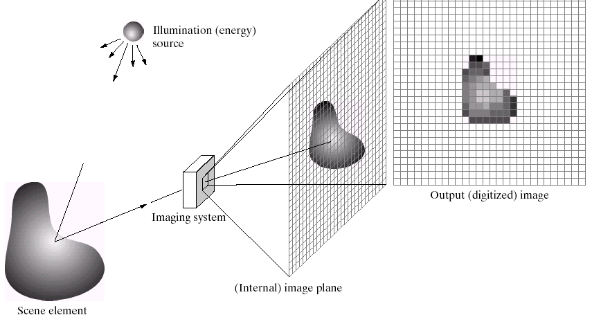
A digital image is a two-dimensional function f(x,y) which the value or amplitude of f(x,y) stands for intensity at spatial coordinates (x,y). As you might be aware, we use RGB (Red, Grey and Blue) color space in common but there are also other color spaces used in image processing. You can find more information about color space and transformation here.
Image Representation
Before we discuss image acquisition recall that a digital image is composed of M rows and N columns of pixels each storing a discrete value. Pixel values are most often gray levels in the range 0 255 (8 bit). Images can easily be represented as matrices.
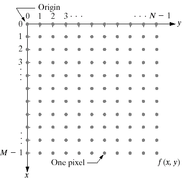
Therefore, we can think about image gray level values in the range [0, 255]
- where 0 is black and 255 is white.
There is no reason why we have to use this range.
- The range [0, 255] stems from display technologies.
For some of the image processing operations gray levels are assumed to be NORMALIZED with 255 and given in the range [0.0, 1.0].
Spatial & Frequency Domains
Image enhancement is the process of making images
more useful. The process is done in different areas with different reasons. In this series, we will focus deeply to understand the logic behind it. The reasons for doing this include:
- Highlighting interesting details in images
- Sharper edges
- Removing noise from images
- Making images more visually appealing.
The main approach is done in spatial and frequency domains. If you are aware of these two, you can skip this subhead. If not, let’s check two broad categories of image enhancement techniques
Spatial domain techniques
- Direct manipulation of image pixels
Frequency domain techniques
- Manipulation of Fourier transform or Wavelet transform or DCT or DFT of an image
For the moment we will concentrate on techniques that operate in the spatial domain.
Image Histograms
An image histogram is a graphical representation of the number of pixels in an image as a function of their intensity.
Histograms are made up of bins, each bin representing a certain intensity value range. The histogram is computed by examining all pixels in the image and assigning each to a bin depending on the pixel intensity. The final value of a bin is the number of pixels assigned to it. The number of bins in which the whole intensity range is divided is usually in the order of the square root of the number of pixels.
Consider an image whose pixel values are confined to some specific range of values only. For eg, brighter images will have all pixels confined to high values. But a good image will have pixels from all regions of the image. So you need to stretch this histogram to either end (as given in the image below, from wikipedia) and that is what Histogram Equalization does (in simple words). This normally improves the contrast of the image.
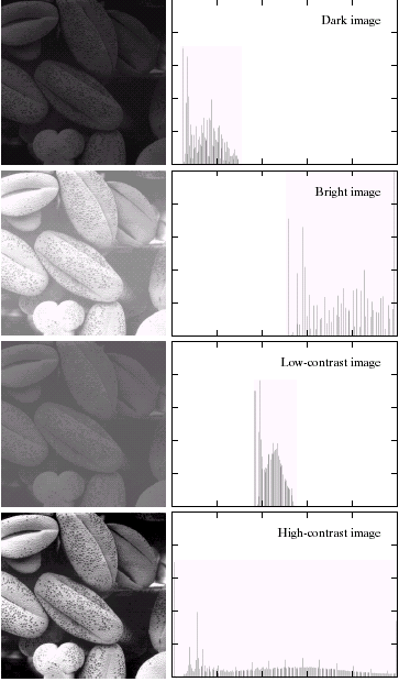
In the example above, notice the relationships between the images and their histograms. We can use this information to enhance the last (high-contrast image). To do so, we will use OpenCV.
import cv2
import numpy as np
from matplotlib import pyplot as plt
img = cv2.imread('wiki.jpg',0)
hist,bins = np.histogram(img.flatten(),256,[0,256])
cdf = hist.cumsum()
cdf_normalized = cdf * hist.max()/ cdf.max()
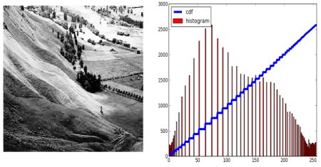
plt.plot(cdf_normalized, color = 'b')
plt.hist(img.flatten(),256,[0,256], color = 'r')
plt.xlim([0,256])
plt.legend(('cdf','histogram'), loc = 'upper left')
plt.show()
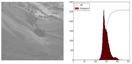
You can see histogram lies in a brighter region. We need the full spectrum. For that, we need a transformation function which maps the input pixels in brighter regions to output pixels in full regions. That is what histogram equalization does.
Now we find the minimum histogram value (excluding 0) and apply the histogram equalization equation. Although, I have used the masked array concept array from Numpy. For a masked array, all operations are performed on non-masked elements. You can read more about it from Numpy docs on masked arrays.
cdf_m = np.ma.masked_equal(cdf,0)
cdf_m = (cdf_m - cdf_m.min())*255/(cdf_m.max()-cdf_m.min())
cdf = np.ma.filled(cdf_m,0).astype('uint8')
Now we have the look-up table that gives us the information on what is the output pixel value for every input pixel value. So we just apply the transform.
img2 = cdf[img]
Another important feature is that, even if the image was a darker image (instead of a brighter one we used), after equalization we will get almost the same image as we got. As a result, this is used as a “reference tool” to make all images with the same lighting conditions. This is useful in many cases. For example, in face recognition, before training the face data, the images of faces are histogram equalized to make them all with the same lighting conditions.